Some users of the MYRLIN#3 model have wondered about the behaviour of the model when very long term projections are made.
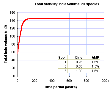
A graph can be made of the total standing volume per ha from column B of Table1. This allows the behaviour of the model to be seen when projections are made without harvesting. The graph at the right shows a projection with three species, with different diameter increment rates(Dinc, cm/yr) but the same mortality rate (AMR, %/yr). The model reaches an equilibrium after about 100 years, which remains constant thereafter.
However, if the mortality rates are made slightly different, as in the example at the left, then the long term equilibrium apparently disappears, and the model in this case shows a continuing decline, without reaching a stable state after 1000 years. Is this a bug in the model? What is actually happening?
The answer lies in the way recruitment is apportioned among species by the model. If a species has higher mortality, its proportion of recruitment will gradually decline relative to other species. Over very long projections, the species with highest mortality will disappear. In this case, the highest mortality is associated with the fastest growing species, so that as it declines, the equilibrium volume also declines. This process simulates the effect of ecological succession. Species with higher mortality rates are shorter lived, and will die out, to be replaced in the population by the slower growing species, even if their proportions are initially quite small.
 A graph can be made of the total standing volume per ha from column B of Table1. This allows the behaviour of the model to be seen when projections are made without harvesting. The graph at the right shows a projection with three species, with different diameter increment rates(Dinc, cm/yr) but the same mortality rate (AMR, %/yr). The model reaches an equilibrium after about 100 years, which remains constant thereafter.
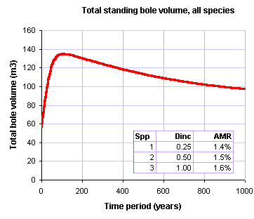 However, if the mortality rates are made slightly different, as in the example at the left, then the long term equilibrium apparently disappears, and the model in this case shows a continuing decline, without reaching a stable state after 1000 years. Is this a bug in the model? What is actually happening?